2. Strong and Weak Form of Linear Elasticity Equivalence

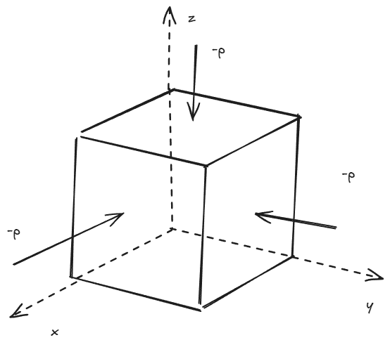
The weak (variational) form follows from the strong equilibrium equations by testing with virtual displacements and integrating by parts. Use it as the blueprint of a finite-element implementation: it fixes the trial and test spaces, the bilinear form and the Neumann terms.

Reading time

4 min

Length

696 words

Updated

Sep 15, 2026

Total views

--

#mechanics/Cauchy-stress#mechanics/hooks-law#mechanics/linear-elasticity

The weak formulation of elasticity is fundamental to the finite-element analysis of ordinary, lattice, and homogenized structures. The weak form is also the basic for implementing the form in the FEniCSx

(1) Kinematics and constitutive equation

Let $\mathrm{\Omega }\subset {\mathbb{R}}^d$, with $d=2$ or $3$, be the reference domain, and let $u:\mathrm{\Omega }\to {\mathbb{R}}^d$ be the displacement field. A material point initially at $x$ moves to $x+u(x)$, so the deformation gradient is

$$\begin{array}{}\text{(1.1)}& F=\frac{\partial u_{new}}{\partial x}=I+\mathrm{\nabla }u.\end{array}$$

The Green--Lagrange strain is

$$\begin{array}{}\text{(1.2)}& E(u)=\frac{1}{2}(F^{T}F-I)=\frac{1}{2}(\mathrm{\nabla }u+\mathrm{\nabla }{u}^T+\mathrm{\nabla }{u}^T\mathrm{\nabla }u).\end{array}$$

Under the small-displacement-gradient assumption, the quadratic term is neglected. This gives the linearized strain tensor

$$\begin{array}{}\text{(1.3)}& \epsilon (u)=\frac{1}{2}(\mathrm{\nabla }u+\mathrm{\nabla }{u}^T)=\mathrm{sym}(\mathrm{\nabla }u).\end{array}$$

The linear constitutive equation is :

$$\begin{array}{}\text{(1.4)}& \sigma (u)=\mathbb{C}:\epsilon (u),{\sigma }_{ij}=C_{ijkl}{\epsilon }_{kl}(u),\end{array}$$

where $\sigma$ is the Cauchy stress and $\mathbb{C}$ is the fourth-order stiffness tensor, with units of Pa. Its inverse, when it exists, is the compliance tensor and has units of ${\text{Pa}}^{-1}$.^[1]

For an isotropic material,

$$\begin{array}{}\text{(1.5)}& \mathbb{C}:\xi =2\mu \xi +\lambda \mathrm{tr}(\xi )I,\end{array}$$

and therefore

$$\begin{array}{}\text{(1.6)}& \sigma (u)=2\mu \epsilon (u)+\lambda \mathrm{tr}(\epsilon (u))I.\end{array}$$

For classical linear elasticity, We know that a stiffness tensor for general material has both minor symmetries major symmetry^[2]:

$$\begin{array}{}\text{(1.7)}& C_{ijkl}=C_{jikl}=C_{ijlk}=C_{klij}.\end{array}$$

(2) Strong form of Linear Elasticity

Split the boundary into a displacement boundary ${\mathrm{\Gamma }}_D$ and a traction boundary ${\mathrm{\Gamma }}_N$:

$$\begin{array}{}\text{(2.1)}& \partial \mathrm{\Omega }=\overline{{\mathrm{\Gamma }}_D\cup {\mathrm{\Gamma }}_N},{\mathrm{\Gamma }}_D\cap {\mathrm{\Gamma }}_N=\varnothing .\end{array}$$

Let $n$ be the outward unit normal, $f$ the body-force density, $u_D$ the prescribed displacement, and $g$ the prescribed traction. Static balance of linear momentum is

$$\begin{array}{}\text{(2.2)}& \boxed{{\displaystyle -\mathrm{\nabla }\cdot \sigma =f\text{in }\mathrm{\Omega },}}\end{array}$$

where, in index notation,

$$\begin{array}{}\text{(2.3)}& -(\mathrm{\nabla }\cdot \sigma {)}_i=-\frac{\partial {\sigma }_{ij}}{\partial x_j}=f_i.\end{array}$$

Strong form of linear elasticity Find $u$ such that

$$\begin{array}{}\text{(strong-form-of-linear-elasticity)}& \{\begin{array}{ll}-\mathrm{\nabla }\cdot (\mathbb{C}:\epsilon (u))=f& \text{in }\mathrm{\Omega },\\ u=u_D& \text{on }{\mathrm{\Gamma }}_D,\\ (\mathbb{C}:\epsilon (u))n=g& \text{on }{\mathrm{\Gamma }}_N.\end{array}\end{array}$$

Where $g$ is the traction applied on the pressure boundaries.

The homogeneous displacement condition used in many examples is the special case $u_D=0$. TopCut,^[3] for example, uses the same equilibrium equation with $f=0$.

(3) Derivation of the weak form

The unknown $u$ is the trial function. Let $v$ be an arbitrary test function that vanishes on the displacement boundary:

$$\begin{array}{}\text{(3.1)}& v=0\text{on }{\mathrm{\Gamma }}_D.\end{array}$$

Multiply the equilibrium equation by $v$ and integrate over $\mathrm{\Omega }$:

$$\begin{array}{}\text{(3.2)}& {\int }_{\mathrm{\Omega }}-(\mathrm{\nabla }\cdot \sigma )\cdot vd\mathrm{\Omega }={\int }_{\mathrm{\Omega }}f\cdot vd\mathrm{\Omega }.\end{array}$$

Integration by parts (the divergence theorem) gives :

$$\begin{array}{}\text{(3.3)}& {\int }_{\mathrm{\Omega }}-(\mathrm{\nabla }\cdot \sigma )\cdot vd\mathrm{\Omega }={\int }_{\mathrm{\Omega }}\sigma :\mathrm{\nabla }vd\mathrm{\Omega }-{\int }_{\partial \mathrm{\Omega }}(\sigma n)\cdot vd\mathrm{\Gamma }.\end{array}$$

This follows component-wise from:

$$\begin{array}{}\text{(3.4)}& \frac{\partial }{\partial x_j}({\sigma }_{ij}{v}_i)=\frac{\partial {\sigma }_{ij}}{\partial x_j}{v}_i+{\sigma }_{ij}\frac{\partial v_i}{\partial x_j}.\end{array}$$

Because $\sigma$ is symmetric, it is orthogonal to the skew-symmetric part of $\mathrm{\nabla }v$. Hence

$$\begin{array}{}\text{(3.5)}& \sigma :\mathrm{\nabla }v=\sigma :\epsilon (v).\end{array}$$

The boundary term splits over ${\mathrm{\Gamma }}_D$ and ${\mathrm{\Gamma }}_N$. On ${\mathrm{\Gamma }}_D$, $v=0$; on ${\mathrm{\Gamma }}_N$, $\sigma n=g$. Consequently,

$$\begin{array}{}\text{(3.6)}& {\int }_{\mathrm{\Omega }}\sigma (u):\epsilon (v)d\mathrm{\Omega }={\int }_{\mathrm{\Omega }}f\cdot vd\mathrm{\Omega }+{\int }_{{\mathrm{\Gamma }}_N}g\cdot vd\mathrm{\Gamma }.\end{array}$$

Substituting $\sigma (u)=\mathbb{C}:\epsilon (u)$ yields the weak equation

$$\begin{array}{}\text{(3.7)}& \boxed{{\displaystyle {\int }_{\mathrm{\Omega }}\epsilon (v):\mathbb{C}:\epsilon (u)d\mathrm{\Omega }={\int }_{\mathrm{\Omega }}f\cdot vd\mathrm{\Omega }+{\int }_{{\mathrm{\Gamma }}_N}g\cdot vd\mathrm{\Gamma }.}}\end{array}$$

(4) Function spaces and weak problem

The trial and test spaces are different when the prescribed displacement is nonzero:

$$\begin{array}{}\text{(4.1)}& U=\{u\in [H^1(\mathrm{\Omega }){]}^d:u{|}_{{\mathrm{\Gamma }}_D}=u_D\},\end{array}$$

$$\begin{array}{}\text{(4.2)}& V=\{v\in [H^1(\mathrm{\Omega }){]}^d:v{|}_{{\mathrm{\Gamma }}_D}=0\}.\end{array}$$

If $u_D=0$, then $U=V$. The requirement $v=0$ applies only on ${\mathrm{\Gamma }}_D$, not on the entire boundary; otherwise the applied traction on ${\mathrm{\Gamma }}_N$ would disappear from the formulation.

[!theorem] Weak form of linear elasticity Find $u\in U$ such that, for every $v\in V$,

$$\begin{array}{}\text{(weak-form-of-linear-elasticity)}& \boxed{{\displaystyle {\int }_{\mathrm{\Omega }}\epsilon (v):\mathbb{C}:\epsilon (u)d\mathrm{\Omega }={\int }_{\mathrm{\Omega }}f\cdot vd\mathrm{\Omega }+{\int }_{{\mathrm{\Gamma }}_N}g\cdot vd\mathrm{\Gamma }}}.\end{array}$$

Equivalently, define

$$\begin{array}{}\text{(4.3)}& a(u,v)={\int }_{\mathrm{\Omega }}\epsilon (v):\mathbb{C}:\epsilon (u)d\mathrm{\Omega },\end{array}$$

and

$$\begin{array}{}\text{(4.4)}& \ell (v)={\int }_{\mathrm{\Omega }}f\cdot vd\mathrm{\Omega }+{\int }_{{\mathrm{\Gamma }}_N}g\cdot vd\mathrm{\Gamma }.\end{array}$$

Then the problem is simply

$$\begin{array}{}\text{(4.5)}& a(u,v)=\ell (v)\text{for every }v\in V.\end{array}$$

(5) Index notation and simplification

Equation $\text{(4.3)}$ can be written as

$$\begin{array}{}\text{(5.1)}& {\int }_{\mathrm{\Omega }}{C}_{ijkl}{\epsilon }_{kl}(u){\epsilon }_{ij}(v)d\mathrm{\Omega }={\int }_{\mathrm{\Omega }}{f}_i{v}_{i}d\mathrm{\Omega }+{\int }_{{\mathrm{\Gamma }}_N}{g}_i{v}_{i}d\mathrm{\Gamma }.\end{array}$$

Using

$$\begin{array}{}\text{(5.2)}& {\epsilon }_{kl}(u)=\frac{1}{2}(\frac{\partial u_k}{\partial x_l}+\frac{\partial u_l}{\partial x_k}),\end{array}$$

and the minor symmetry $C_{ijkl}=C_{ijlk}$,

$$\begin{array}{}\text{(5.3)}& \begin{array}{rl}{C}_{ijkl}{\epsilon }_{kl}(u)& =\frac{1}{2}{C}_{ijkl}\frac{\partial u_k}{\partial x_l}+\frac{1}{2}{C}_{ijkl}\frac{\partial u_l}{\partial x_k}\\ & =\frac{1}{2}{C}_{ijkl}\frac{\partial u_k}{\partial x_l}+\frac{1}{2}{C}_{ijlk}\frac{\partial u_k}{\partial x_l}\\ & =C_{ijkl}\frac{\partial u_k}{\partial x_l}.\end{array}\end{array}$$

Applying the other minor symmetry to the test-function gradient gives the equivalent expression

$$\begin{array}{}\text{(5.4)}& \boxed{{\displaystyle {\int }_{\mathrm{\Omega }}{C}_{ijkl}\frac{\partial u_k}{\partial x_l}\frac{\partial v_i}{\partial x_j}d\mathrm{\Omega }={\int }_{\mathrm{\Omega }}{f}_i{v}_{i}d\mathrm{\Omega }+{\int }_{{\mathrm{\Gamma }}_N}{g}_i{v}_{i}d\mathrm{\Gamma }}}.\end{array}$$

For a perforated or heterogeneous microscopic domain ${\mathrm{\Omega }}^{\epsilon }$, as commonly used for lattice structures and homogenization, replace $\mathrm{\Omega }$ by ${\mathrm{\Omega }}^{\epsilon }$ and use its corresponding boundary partition. The derivation is otherwise unchanged.

---

1. Constitutive equation ↩︎

2. 1. Symmetric Stiffness Tensor and Voigt notation ↩︎

3. Andreasen, Casper Schousboe, Martin Ohrt Elingaard, and Niels Aage. “Level Set Topology and Shape Optimization by Density Methods Using Cut Elements with Length Scale Control.” Structural and Multidisciplinary Optimization 62, no. 2 (2020): 685–707. https://doi.org/10.1007/s00158-020-02527-1. ↩︎